Much of statistics and econometrics literature has evolved around time-series type of data. We deal with such data sets in various areas such as weather prediction, stock market, and macroeconomics. Unemployment rate, temperature, price of stock or commodities are all examples of values that we observe through time. And, collection of any of those values by intervals in a window of time would assemble a time-series of those values by those intervals in the observed time window. In this series of posts, we consider proper tools and best practices with regard to analyzing time-series. We will also present real cases and examples using introduced methodologies in each post.
In this initial post, we focus on the topic of cointegration and show how the Fed, using the same practices, can use it to predict quarterly issued consumer loan charge-off rate.
COINTEGRATION DEFINED
In order to explain cointegration, we must first consider the concept of stationary time-series. In short, a stationary variable varies around a constant mean with a constant variance. For instance let’s look at US GDP for about the past 15 years:
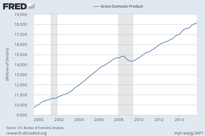
As we can see in the above graph, the mean and variance of the variable we observe in that time window are changing and, in general, increasing as time goes forward. Hence, we can state that we see a non-stationary pattern in time-series of US GDP from 2000 to 2015. However, if we look at growth rate (i.e. the difference in GDP between consecutive years), then we have a stationary variable as mean and variance stay fairly constant through different points of time in the time window as seen in the following graph:
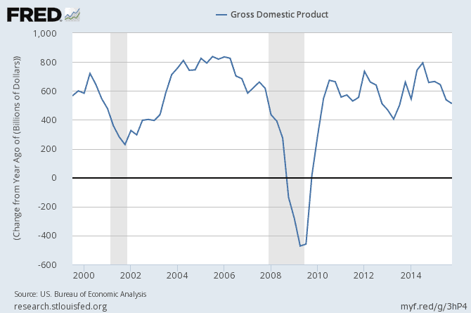
In this example, US GDP is a time-series with order of integration of one. By definition, the number of times that we have to differentiate a time-series variable to reach a stationary process is the order of integration of that time-series variable. Thus, the order of integration for US GDP growth rate from 2000 to 2015 is zero. Usually, working with non-stationary data, integrated by order higher than zero, could end up in spurious regression results. We will talk about spurious regression in time-series in upcoming posts. In the meantime, you’ll find interesting spurious correlation examples in this website:
http://tylervigen.com/spurious-correlations
Finally, we come to the definition of cointegration! Two time series are cointegrated if:
1.They are both integrated of order one
2.The error term from the best linear model between the two series is stationary
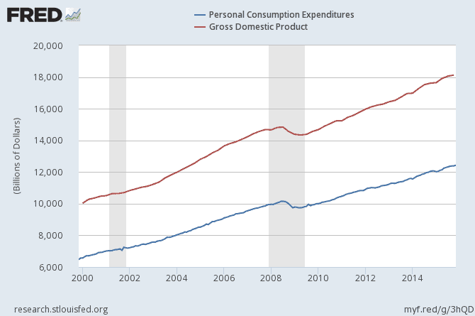
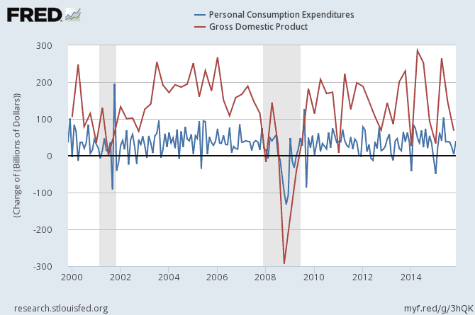
The second condition considers whether the two time series move together or if their trends are completely irrelevant. If the two time series have similar stochastic trends in the background, that trend will be eliminated in the linear model between the two time-series and the residuals will be stationary. For instance, number of alcohol related deaths in Scotland is an integrated order of one. But, US GDP and number of alcohol related deaths in Scotland are not cointegrated as their stochastic trends are not relative and do not cancel each other out in a linear model between the two time-series. Hence, the error term of that model is non-stationary and the two time-series are not cointegrated. On the other hand, US personal consumption expenditures and US GDP growth is an example of two cointegrated time-series. We can see this in the following graphs. Sometimes, we do not really have to run statistical tests, as graphs would clearly lead us to the right inference.
ERROR CORRECTION MODEL
When we deal with cointegrated time-series, use of error correction model (ECM) technique is recommended. For instance, if we want to model Personal Consumption Expenditure using GDP, then we deal with two cointegrated time-series. Only using the non-stationary (original values) variables, we will have a biased model due to ignored dynamics. In such cases, our models are only good for long-run relationships. Let’s review the steps in ECM modeling:
Assuming we want to model variable Yt using Xt where Y and X are cointegrated time-series:
1.Acquire, et, error terms from the linear model between Y and X: Yt = α + βXt + et
2.Difference consecutive values in each series to create new series of ΔYt and ΔXt where ΔYt = Yt – Yt-1
3.Find a linear model of ΔYt using ΔXt and et-1 as explanatory variables.
Since in ECM, we deal with non-stationary variables, our model actually describes the short-term relationships between the growth rates of our cointegrated time-series. Besides, et-1, which is the reason behind the naming of the model, corrects our interpretation by the long-run relationship between our cointegrated time-series. In summary there are two main takeaways from using ECM models when dealing with cointegrated time-series:
1.Linear representation of relationship between cointegrated time-series is biased while ECM does not suffer from the same problem.
2.ECM models are robust as they account for both long run and short-run relations.
Hence, it is strongly recommended to use ECM models rather than ordinary linear models when dealing with cointegrated variables and non-stationary data.
ECM USE CASE EXAMPLE
Using the ECM framework, we built a predictive model for quarterly issued consumer loan charge-off rate by Fed. Right now, our model predicts that rate by two quarters ahead in time, and, based on different scenarios, it could extend the prediction window and give us longer projections. As we were dealing with cointegrated time series, we knew that ECM is the way to go compared to ordinary linear models, LM. (NOTE: proprietary agreements prohibit us from naming the explanatory variables used in our model). But, for the purpose of this post, we’ll share the performance of ECM and LM in predicting the consumer loan charge-off rate in the case. The first graph here shows the historical actual values of charge-off rates, which are seasonally adjusted, along with the fitted values for those rates from ECM and LM models. LM and ECM values are dotted for 2015 reported quarters since we left those three quarters out of our model creation phase. So, we could compare models’ performances on the observed values that were not used in model creation.
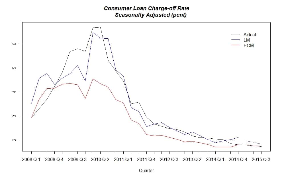
As you see in the graph, the blue line, LM, seems to be a better overall fit (long-run). But, in the 2015 quarters it is ECM that performs much better than LM. In fact the ECM’s Root Mean Squared Forecast Error in our hold up sample, 2015 quarters, is about 40 times less than that of LM. So, our choice as it was predicted is ECM. Now, we use the full range of available data to retool our ECM model and generate our forecast. For the sake of comparison, we also generated LM forecast values. The same three values shown in the previous graph are now updated in the next one:
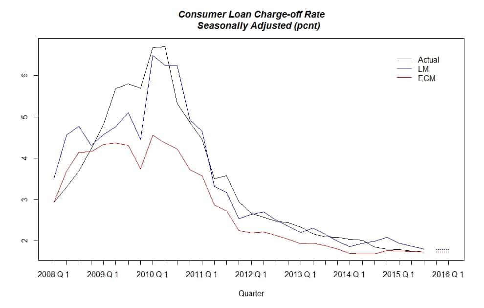
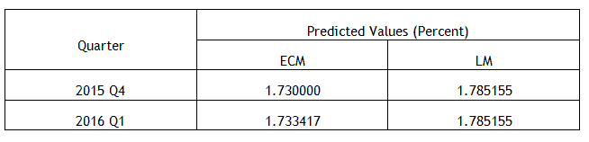
The final reported value of Consumer Loan Charge-off Rate by Fed is 1.73% for the 3rd quarter of 2015. With that in mind, let’s finish this post by presenting our prediction values for the next two quarters.